Test difference between correlation coefficient estimates and a value of reference

This function tests whether smoothed correlation values are equal (H0) or not to a reference value (default = 0). The test is not described in Choi & Shin, 2021, but it is based on the idea behind test_equality().

Usage

test_ref(
  tcor_obj,
  t = tcor_obj$t,
  r_ref = 0,
  test = c("student", "chi2"),
  p.adjust.methods = c("none", "bonferroni", "holm", "hochberg", "hommel", "BH", "BY",
    "fdr")
)

Arguments

tcor_obj: the output of a call to tcor() with CI = TRUE.
t: a vector of time point(s) used by the test (by default, all time points are considered).
r_ref: a scalar indicating the reference value for the correlation coefficient to be used in the test (default = 0).
test: a character string indicating which test to use ("student", the default; or "chi2").
p.adjust.methods: a character string indicating the method used to adjust p-values for multiple testing (see p.adjust(); default = "none").

Value

a data.frame with the result of the test, including the effect size (delta_r = r[t] - r_ref).

Details

Two different test statistics can be used, one is asymptotically Student-t distributed under H0 and one is chi-square distributed. In practice, it seems to give very similar results.

Examples

## Comparison of all correlation values to reference of 0.5

res <- with(stockprice, tcor(x = SP500, y = FTSE100, t = DateID, h = 300, CI = TRUE))
ref <- 0.5
test_against_ref <- test_ref(res, r_ref = ref)
#> The bandwidth stored in `tcor_obj` and used by `test_ref()` has not been automatically selected but was set by the user. Rerun `tcor()` without specifying `h` if you want otherwise.
head(test_against_ref)
#>            t         r r_ref     delta_r SE_delta_r     T_stat   df         p
#> 1 2000-04-03 0.4354187   0.5 -0.06458131 0.07161311 -0.9018084 8650 0.3671838
#> 2 2000-04-04 0.4362800   0.5 -0.06372005 0.07142815 -0.8920859 8650 0.3723717
#> 3 2000-04-05 0.4370884   0.5 -0.06291158 0.07124627 -0.8830157 8650 0.3772523
#> 4 2000-04-06 0.4378701   0.5 -0.06212989 0.07106580 -0.8742587 8650 0.3820017
#> 5 2000-04-07 0.4386006   0.5 -0.06139941 0.07088820 -0.8661442 8650 0.3864351
#> 6 2000-04-10 0.4408871   0.5 -0.05911287 0.07059415 -0.8373622 8650 0.4024122
#>   p_adjustment
#> 1         none
#> 2         none
#> 3         none
#> 4         none
#> 5         none
#> 6         none


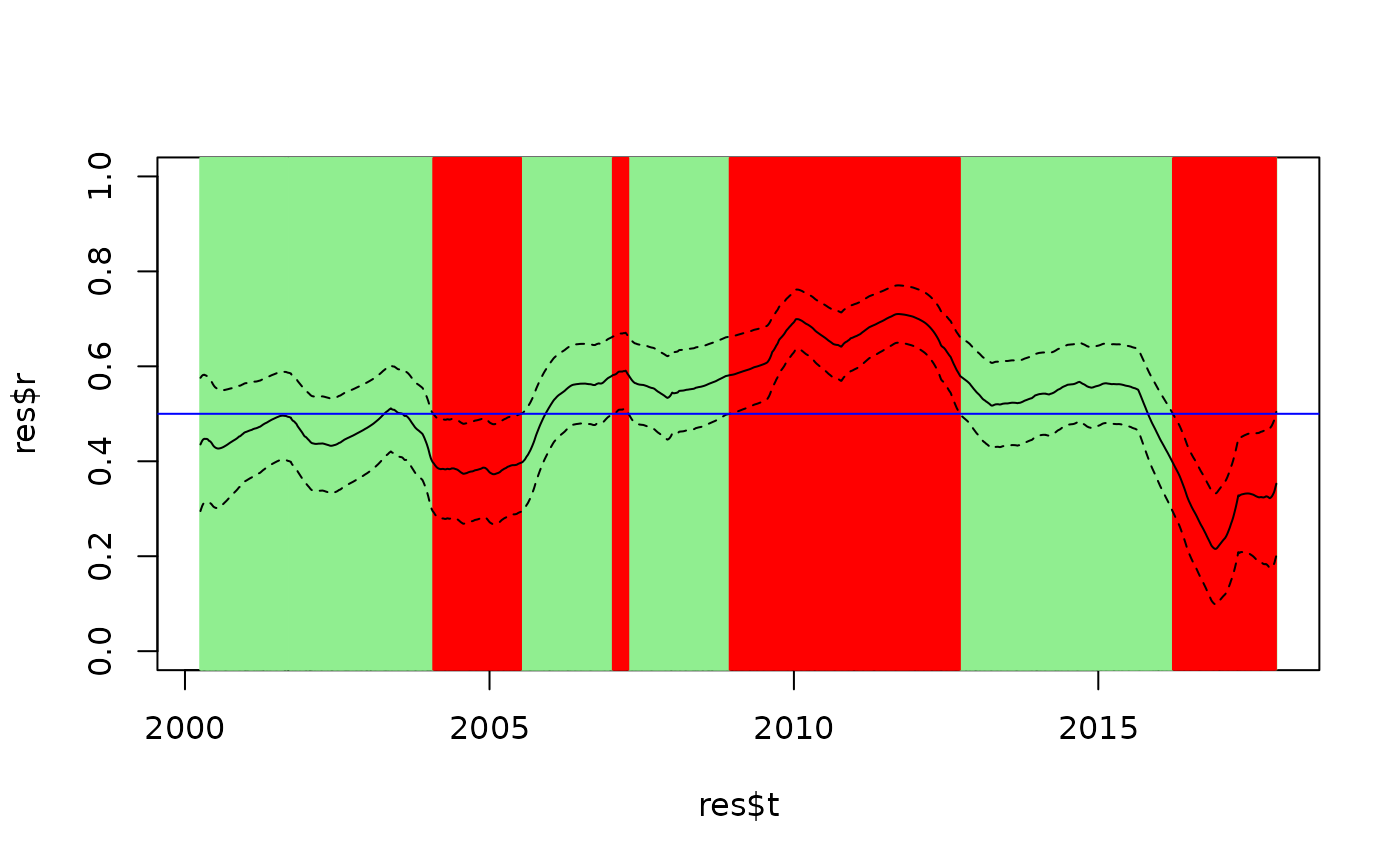
## Plot to illustrate the correspondance with confidence intervals

plot(res$r ~ res$t, type = "l", ylim = c(0, 1), col = NULL)
abline(v = test_against_ref$t[test_against_ref$p > 0.05], col = "lightgreen")
abline(v = test_against_ref$t[test_against_ref$p < 0.05], col = "red")
points(res$r ~ res$t, type = "l")
points(res$upr ~ res$t, type = "l", lty = 2)
points(res$lwr ~ res$t, type = "l", lty = 2)
abline(h = ref, col = "blue")



## Test correlation of 0 a specific time points (using index or dates)

test_ref(res, t = c(100, 150))
#> The bandwidth stored in `tcor_obj` and used by `test_ref()` has not been automatically selected but was set by the user. Rerun `tcor()` without specifying `h` if you want otherwise.
#>     t         r r_ref   delta_r SE_delta_r   T_stat   df            p
#> 1 100 0.4321759     0 0.4321759 0.06039284 7.156078 8650 8.979024e-13
#> 2 150 0.4483478     0 0.4483478 0.05536091 8.098635 8650 6.313458e-16
#>   p_adjustment
#> 1         none
#> 2         none
test_ref(res, t = c("2000-08-18", "2000-10-27"))
#> The bandwidth stored in `tcor_obj` and used by `test_ref()` has not been automatically selected but was set by the user. Rerun `tcor()` without specifying `h` if you want otherwise.
#>            t         r r_ref   delta_r SE_delta_r   T_stat   df            p
#> 1 2000-08-18 0.4300012     0 0.4300012 0.06110005 7.037657 8650 2.104015e-12
#> 2 2000-10-27 0.4455035     0 0.4455035 0.05609660 7.941720 8650 2.243738e-15
#>   p_adjustment
#> 1         none
#> 2         none